Before using this tutorial, we recommend that you read through our introductory tutorial.
Overview
In this tutorial we explore more advanced uses of DiffSegR:
- How to explore a range of segmentation models ?
- How to select a subset of segments whose absolute \(\log_2\)-FC passes a threshold while keeping statistical guarantees on the true discovery proportion in this subset ? (Post hoc inference)
Exploring more segmentations
After visual inspection, one can disagree with the segmentation of the \(\log_2\)-FC proposed by DiffSegR. It can happen when spurious changepoints, resulting from an over-segmentation of the \(\log_2\)-FC, seems to be added. In this case it is often useful to explore several different segmentations in order to choose a more suitable hyperparameter \(\alpha\) value.
To explore all reachable segmentations between 1 to Kmax segments, one can pass segmentNeighborhood = TRUE and specify the value of Kmax to segmentationLFC(). This step can be time consuming. A grid search approach is also implemented in DiffSegR (see gridSearch and alphas parameters of segmentationLFC()).
features <- segmentationLFC(
  data                = data,
  outputDirectory     = working_directory,
  segmentNeighborhood = TRUE,
  Kmax                = 50
)
#>
#>  > Segmenting the log2-FC of locus ChrC 71950-78500 (ID : psbB_petD) ...
#>
#>  > Finished in 0.873086214065552 secs
The figures showing the path of all reachable segmentations up to Kmax segments of the log2-FC on reverse and forward strands are accessible in the working directory under the name all_models_minus.rds and all_models_plus.rds.
A good practice is to select a robust segmentation. Visually it is equivalent to pick the elbow of this curve. In this example we can select \(\alpha=5.46\) symbolized by the red line.
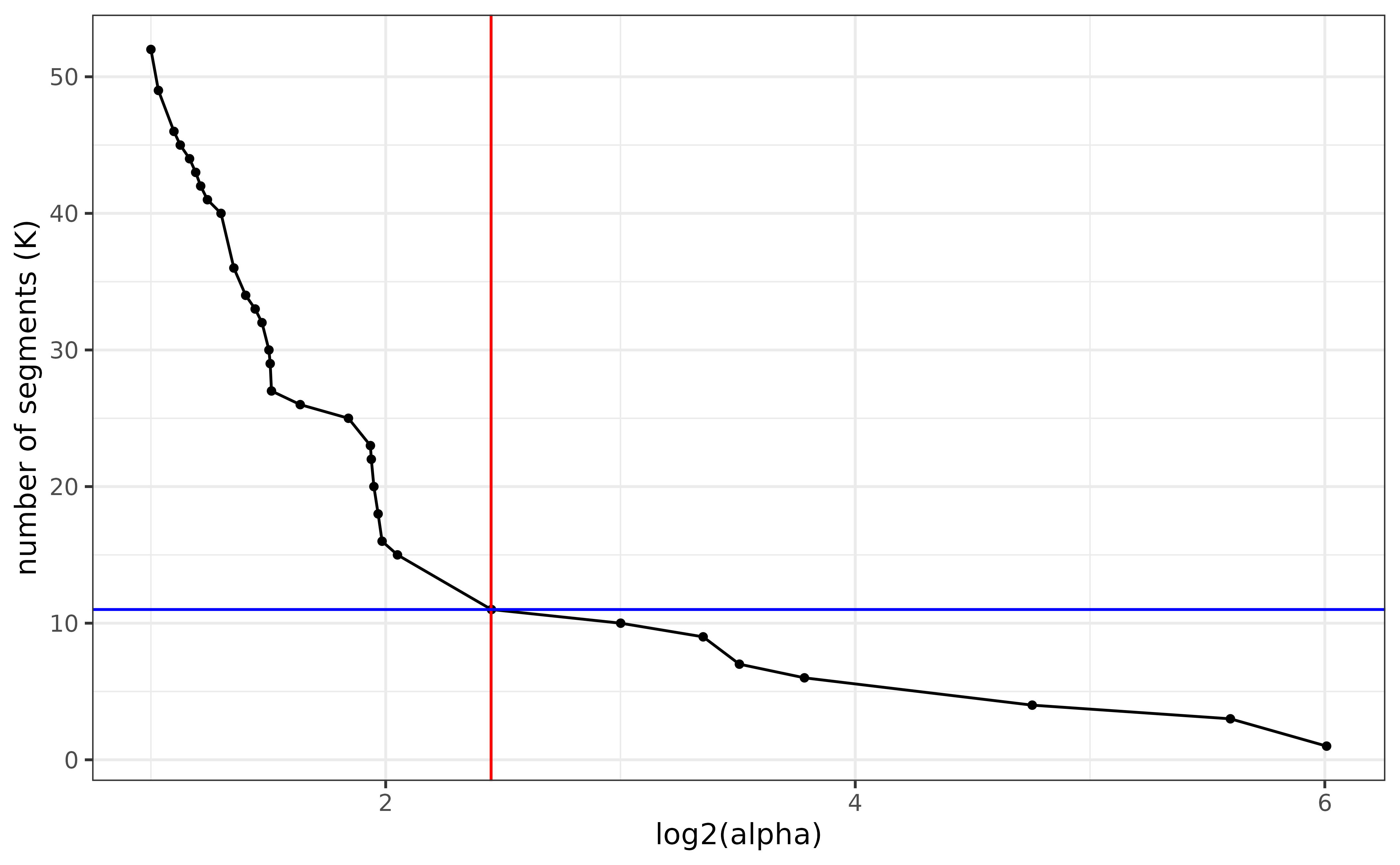
Path of all reachable segmentations up to 50 segments of the log2-FC on reverse strand. Corresponding alpha values on the log scale can be read on X-axis.
Post hoc inference
If the result of the DEA does not correspond to what the user expected, they may tend to snoop in the data and eventually select a subset of segments of interest. For instance it is a common usage to define a threshold on the absolute \(\log_2\)-FC per-segment. In this case DiffSegR will declare differentially expressed the largest set of segments with an absolute \(\log_2\)-FC > threshold and a true discovery proportion lower bound choose by the user (postHoc_tdpLowerBound). This post-hoc lower bound is obtained by controlling the joint error rate (JER) using the Simes family of thresholds (Blanchard et al. 2020).
To use post hoc inference one have to specify :
- its decision rule, i.e a predicate function that returns a single
TRUEorFALSEif the segment on which it is applied meets the conditions defined in the predicate. The criteria used in the predicate have to be defined for each segment inSummarizedExperiment::mcols(dds). Here,predicate = function(x) 2^abs(x$log2FoldChange)>2; - the minimum true discovery proportion among the subset of segments declared differentially expressed. Here,
postHoc_tdpLowerBound = 0.05; - the significance level of the test procedure. Here,
postHoc_significanceLevel = 0.05.
dds <- dea(
  SExp                      = SExp,
  design                    = ~ condition,
  sizeFactors               = rep(1,4),
  predicate                 = function(x) 2^abs(x$log2FoldChange)>2,
  postHoc_significanceLevel = 0.05,
  postHoc_tdpLowerBound     = 0.95
)
#>
#>  > differential expression analysis ...
#> renaming the first element in assays to 'counts'
#> gene-wise dispersion estimates
#> mean-dispersion relationship
#> final dispersion estimates
#>
#>  > multiple testing correction ...
#>
#>  > postHoc selection ...
#>
#>  > 37 DERs with at least 0.972972972972973 of true positives.
#- check fold-change of differentially expressed segments ---------------------#
DERs <- dds[SummarizedExperiment::mcols(dds)$DER,]
2^abs(SummarizedExperiment::mcols(DERs)$log2FoldChange)
#>  [1]  2.122779  2.034771  2.320207  3.351678  3.807408  4.991526 24.968252
#>  [8] 15.124988  5.923075 20.499897 13.499973 14.499983 13.999986 13.428559
#> [15] 11.714275 23.999928 23.333263 17.666614 19.499904  2.655736  3.096773
#> [22]  2.999999  3.194028  3.246375  3.140844  3.140844  3.531248  3.328357
#> [29]  3.903844  3.784312  3.784312  4.062498  3.686272  4.351348  4.548383
#> [36]  4.187497  5.470581
References
Blanchard, G., Neuvial, P. and Roquain, E. Post hoc confidence bounds on false positives using reference families. Ann. Statist 48(3), 1281-1303 (2020) doi.org/10.1214/19-AOS1847.