Tutorial : Transcriptome-Wide Differential Expression Analysis with DiffSegR
Source:vignettes/introductory_tutorial.Rmd
introductory_tutorial.RmdData
In this tutorial we use an RNA-Seq dataset (SRA046998) generated to study the differences in Arabidopsis thaliana chloroplast RNA metabolism between a control (wt) and a null mutant of the chloroplast-targeted \(3'\to5'\) exoribonuclease polynucleotide phosphorylase (pnp1-1). In comparison to control plants, this mutant overaccumulate RNA fragments that are mainly located outside of the annotated genic areas and the RNA-Seq data have been extensively validated using molecular techniques (Castandet et al. 2013; Hotto et al. 2015). Both conditions contain two biological replicates. Only a diluted set of reads overlapping positions 71950 to 78500 on chloroplast genome has been kept as a minimal dataset example.
Overview
After setting up the necessary working environnement and loading the software, we are going through each step of a classical differential expression analysis along the genome with DiffSegR:
- Definition of the experiment and calculation of coverages from bam files ;
- Summarize the differential transcription landscape, i.e. (i) identify segments along the genome in the per-base \(\log_2\)-FC and (ii) count reads overlapping them ;
- Use the counts as measures of the expression abundance of the segments for differential expression analysis ;
- Annotate the differential expressed regions (DERs) ;
- Visualize the DERs.
Setup
First, we create a working directory that will host all the files produced by DiffSegR during the analysis (coverages, results).
working_directory <- "./DIFFSEGR_TEST"
dir.create(working_directory, showWarnings = FALSE)
Then, we save sample information that we will use for this tutorial in a data.frame. In practice, one can create the working directory and write the text file by hand. The sample information file needs to include the following columns:
- sample : identifier for the sample ;
- condition : identifier for the condition ;
- replicate : identifier for the replicate ;
- bam : path to the bam file (.bam) ;
- isPairedEnd : logical indicating if the library contain paired-end reads or not (TRUE/FALSE) ;
- strandSpecific : integer indicating if a strand-specific analysis should be performed. 0 (unstranded), 1 (stranded) and 2 (reversely stranded). WARNING: All samples must be consistently stranded or non-stranded. Ensure uniformity across your dataset to avoid analysis errors.
Note: Coverages are computed internally by DiffSegR from bam files and saved in rds format at the location specified by the user (coverage column).
#- create sample information table --------------------------------------------#
sample_info <- data.frame(
  sample    = c("pnp1_1_1", "pnp1_1_2", "wt_1", "wt_2"),
  condition = rep(c("pnp1_1", "wt"), each = 2),
  replicate = rep(1:2,2),
  bam       = sapply(
    c("pnp1_1_1_ChrC_71950_78500.bam",
      "pnp1_1_2_ChrC_71950_78500.bam",
      "wt_1_ChrC_71950_78500.bam",
      "wt_2_ChrC_71950_78500.bam"
    ),
    function(bam) system.file("extdata", bam, package = "DiffSegR")
  ),
  isPairedEnd    = rep(FALSE, 4),
  strandSpecific = rep(1, 4)
)

#- display sample information table -------------------------------------------#
knitr::kable(sample_info, row.names = FALSE)| sample | condition | replicate | bam | isPairedEnd | strandSpecific |
|---|---|---|---|---|---|
| pnp1_1_1 | pnp1_1 | 1 | /tmp/Rtmpmuyfvl/temp_libpath1d15a968813/DiffSegR/extdata/pnp1_1_1_ChrC_71950_78500.bam | FALSE | 1 |
| pnp1_1_2 | pnp1_1 | 2 | /tmp/Rtmpmuyfvl/temp_libpath1d15a968813/DiffSegR/extdata/pnp1_1_2_ChrC_71950_78500.bam | FALSE | 1 |
| wt_1 | wt | 1 | /tmp/Rtmpmuyfvl/temp_libpath1d15a968813/DiffSegR/extdata/wt_1_ChrC_71950_78500.bam | FALSE | 1 |
| wt_2 | wt | 2 | /tmp/Rtmpmuyfvl/temp_libpath1d15a968813/DiffSegR/extdata/wt_2_ChrC_71950_78500.bam | FALSE | 1 |
Analysis
Now, we present a basic use of the main functions of the DiffSegR R package. Our focus is on analyzing the sequence stretch from positions 71950 to 78500 in the chloroplast genome (ChrC). This locus corresponds to the polycistronic gene cluster from psbB to petD. To optimize processing, we’ll allocate 4 logical cores for examining this locus. Users have the flexibility to adjust this setting based on their available computational resources. Additionally, it’s possible to concurrently analyze multiple genomic regions of interest (see our multi-loci analysis tutorial). By doing so, users can efficiently manage the total number of threads for the analysis, as well as how many threads are assigned to each locus. Thus, the ratio of the total number of threads to the number assigned per locus determines the number of locus analyzed simultaneously.
Step 1: Definition of the experiment and calculation of coverages from bam files
newExperiment() imports relevant data about the RNA-Seq samples and a specified locus (e.g., ChrC: 71950 - 78500).
data <- newExperiment(
  sampleInfo   = sample_info,
  loci         = data.frame(
    seqid      = "ChrC",
    chromStart = 71950,
    chromEnd   = 78500,
    locusID    = "psbB_petD"
  ),
  referenceCondition = "wt",
  otherCondition     = "pnp1_1",
  nbThreads          = nb_threads_tot,
  nbThreadsByLocus   = nb_threads_locus,
  coverage           = working_directory
)

print(data)
#> $sampleInfo
#>                                 sample condition replicate
#> pnp1_1_1_ChrC_71950_78500.bam pnp1_1_1    pnp1_1         1
#> pnp1_1_2_ChrC_71950_78500.bam pnp1_1_2    pnp1_1         2
#> wt_1_ChrC_71950_78500.bam         wt_1        wt         1
#> wt_2_ChrC_71950_78500.bam         wt_2        wt         2
#>                                                                                                                  bam
#> pnp1_1_1_ChrC_71950_78500.bam /tmp/Rtmpmuyfvl/temp_libpath1d15a968813/DiffSegR/extdata/pnp1_1_1_ChrC_71950_78500.bam
#> pnp1_1_2_ChrC_71950_78500.bam /tmp/Rtmpmuyfvl/temp_libpath1d15a968813/DiffSegR/extdata/pnp1_1_2_ChrC_71950_78500.bam
#> wt_1_ChrC_71950_78500.bam         /tmp/Rtmpmuyfvl/temp_libpath1d15a968813/DiffSegR/extdata/wt_1_ChrC_71950_78500.bam
#> wt_2_ChrC_71950_78500.bam         /tmp/Rtmpmuyfvl/temp_libpath1d15a968813/DiffSegR/extdata/wt_2_ChrC_71950_78500.bam
#>                               isPairedEnd strandSpecific
#> pnp1_1_1_ChrC_71950_78500.bam       FALSE              1
#> pnp1_1_2_ChrC_71950_78500.bam       FALSE              1
#> wt_1_ChrC_71950_78500.bam           FALSE              1
#> wt_2_ChrC_71950_78500.bam           FALSE              1
#>
#> $referenceCondition
#> [1] "wt"
#>
#> $otherCondition
#> [1] "pnp1_1"
#>
#> $loci
#> GRanges object with 1 range and 1 metadata column:
#>       seqnames      ranges strand |     locusID
#>          <Rle>   <IRanges>  <Rle> | <character>
#>   [1]     ChrC 71950-78500      * |   psbB_petD
#>   -------
#>   seqinfo: 1 sequence from an unspecified genome; no seqlengths
#>
#> $nbThreads
#> [1] 4
#>
#> $nbThreadsByLocus
#> [1] 4
#>
#> $stranded
#> [1] TRUE
#>
#> $coverageDir
#> [1] "./DIFFSEGR_TEST"
coverage() generates coverage profiles from BAM files for the locus of interest. When reads are stranded (stranded = TRUE), it creates a separate coverage profile for each strand across replicates of the biological conditions being compared. By default, coverage is calculated using a geometric mean of the 5’ and 3’ ends of aligned reads (coverageType = "average"). If the coverage is too sparse, one may calculate the coverage based on the entire read by using the argument coverageType = "fullLength".
coverage(
data = data,
coverageType = "average"
)
#>
#> > Calculating coverage of locus ChrC 71950-78500 (ID : psbB_petD) ...
#>
#> ========== _____ _ _ ____ _____ ______ _____
#> ===== / ____| | | | _ \| __ \| ____| /\ | __ \
#> ===== | (___ | | | | |_) | |__) | |__ / \ | | | |
#> ==== \___ \| | | | _ <| _ /| __| / /\ \ | | | |
#> ==== ____) | |__| | |_) | | \ \| |____ / ____ \| |__| |
#> ========== |_____/ \____/|____/|_| \_\______/_/ \_\_____/
#> Rsubread 2.18.0
#>
#> //========================== featureCounts setting ===========================\\
#> || ||
#> || Input files : 4 BAM files ||
#> || ||
#> || pnp1_1_1_ChrC_71950_78500.bam ||
#> || pnp1_1_2_ChrC_71950_78500.bam ||
#> || wt_1_ChrC_71950_78500.bam ||
#> || wt_2_ChrC_71950_78500.bam ||
#> || ||
#> || Paired-end : no ||
#> || Count read pairs : no ||
#> || Annotation : R data.frame ||
#> || Dir for temp files : . ||
#> || Threads : 4 ||
#> || Level : meta-feature level ||
#> || Multimapping reads : counted ||
#> || Multi-overlapping reads : counted ||
#> || Min overlapping bases : 1 ||
#> || Read reduction : to 3' end ||
#> || ||
#> \\============================================================================//
#>
#> //================================= Running ==================================\\
#> || ||
#> || Load annotation file .Rsubread_UserProvidedAnnotation_pid11345 ... ||
#> || Features : 13102 ||
#> || Meta-features : 13102 ||
#> || Chromosomes/contigs : 1 ||
#> || ||
#> || Process BAM file pnp1_1_1_ChrC_71950_78500.bam... ||
#> || Strand specific : stranded ||
#> || Single-end reads are included. ||
#> || Total alignments : 24260 ||
#> || Successfully assigned alignments : 24249 (100.0%) ||
#> || Running time : 0.00 minutes ||
#> || ||
#> || Process BAM file pnp1_1_2_ChrC_71950_78500.bam... ||
#> || Strand specific : stranded ||
#> || Single-end reads are included. ||
#> || Total alignments : 21100 ||
#> || Successfully assigned alignments : 21098 (100.0%) ||
#> || Running time : 0.00 minutes ||
#> || ||
#> || Process BAM file wt_1_ChrC_71950_78500.bam... ||
#> || Strand specific : stranded ||
#> || Single-end reads are included. ||
#> || Total alignments : 17533 ||
#> || Successfully assigned alignments : 17531 (100.0%) ||
#> || Running time : 0.00 minutes ||
#> || ||
#> || Process BAM file wt_2_ChrC_71950_78500.bam... ||
#> || Strand specific : stranded ||
#> || Single-end reads are included. ||
#> || Total alignments : 14070 ||
#> || Successfully assigned alignments : 14066 (100.0%) ||
#> || Running time : 0.00 minutes ||
#> || ||
#> || Write the final count table. ||
#> || Write the read assignment summary. ||
#> || ||
#> \\============================================================================//
#>
#>
#> ========== _____ _ _ ____ _____ ______ _____
#> ===== / ____| | | | _ \| __ \| ____| /\ | __ \
#> ===== | (___ | | | | |_) | |__) | |__ / \ | | | |
#> ==== \___ \| | | | _ <| _ /| __| / /\ \ | | | |
#> ==== ____) | |__| | |_) | | \ \| |____ / ____ \| |__| |
#> ========== |_____/ \____/|____/|_| \_\______/_/ \_\_____/
#> Rsubread 2.18.0
#>
#> //========================== featureCounts setting ===========================\\
#> || ||
#> || Input files : 4 BAM files ||
#> || ||
#> || pnp1_1_1_ChrC_71950_78500.bam ||
#> || pnp1_1_2_ChrC_71950_78500.bam ||
#> || wt_1_ChrC_71950_78500.bam ||
#> || wt_2_ChrC_71950_78500.bam ||
#> || ||
#> || Paired-end : no ||
#> || Count read pairs : no ||
#> || Annotation : R data.frame ||
#> || Dir for temp files : . ||
#> || Threads : 4 ||
#> || Level : meta-feature level ||
#> || Multimapping reads : counted ||
#> || Multi-overlapping reads : counted ||
#> || Min overlapping bases : 1 ||
#> || Read reduction : to 5' end ||
#> || ||
#> \\============================================================================//
#>
#> //================================= Running ==================================\\
#> || ||
#> || Load annotation file .Rsubread_UserProvidedAnnotation_pid11345 ... ||
#> || Features : 13102 ||
#> || Meta-features : 13102 ||
#> || Chromosomes/contigs : 1 ||
#> || ||
#> || Process BAM file pnp1_1_1_ChrC_71950_78500.bam... ||
#> || Strand specific : stranded ||
#> || Single-end reads are included. ||
#> || Total alignments : 24260 ||
#> || Successfully assigned alignments : 24251 (100.0%) ||
#> || Running time : 0.00 minutes ||
#> || ||
#> || Process BAM file pnp1_1_2_ChrC_71950_78500.bam... ||
#> || Strand specific : stranded ||
#> || Single-end reads are included. ||
#> || Total alignments : 21100 ||
#> || Successfully assigned alignments : 21088 (99.9%) ||
#> || Running time : 0.00 minutes ||
#> || ||
#> || Process BAM file wt_1_ChrC_71950_78500.bam... ||
#> || Strand specific : stranded ||
#> || Single-end reads are included. ||
#> || Total alignments : 17533 ||
#> || Successfully assigned alignments : 17520 (99.9%) ||
#> || Running time : 0.00 minutes ||
#> || ||
#> || Process BAM file wt_2_ChrC_71950_78500.bam... ||
#> || Strand specific : stranded ||
#> || Single-end reads are included. ||
#> || Total alignments : 14070 ||
#> || Successfully assigned alignments : 14060 (99.9%) ||
#> || Running time : 0.00 minutes ||
#> || ||
#> || Write the final count table. ||
#> || Write the read assignment summary. ||
#> || ||
#> \\============================================================================//
#>
#> > Finished in 1.25298714637756 secsTo enhance efficiency, users have the option to pre-process by subsetting BAM files to the locus of interest, which can notably reduce running times (refer to subsettingBams parameter in ?DiffSegR::coverage).
coverage(
  data           = data,
  coverageType   = "average",
  subsettingBams = TRUE
)
Setp 2: Summarizing the differential transcription landscape
segmentationLFC() transforms coverage profiles into the per-base \(\log_2\)-FC (one by strand). The reference biological condition specified by the user is set to the denominator (referenceCondition = "wt"). segmentationLFC() then calls fpopw::Fpop_w(), a changepoint detection in the mean of a Gaussian signal approach, on the per-base \(\log_2\)-FC of both strands to retrieve the segments boundaries (changepoints). The hyperparameter \(\alpha\) specified by the user controls the number of returned segments. The number of changepoints is a decreasing function of \(\alpha\). By default alpha=2. The segments are stored as a GRanges object.
features <- segmentationLFC(
  data  = data,
  alpha = 2
)
#>
#>  > Segmenting the log2-FC of locus ChrC 71950-78500 (ID : psbB_petD) ...
#>
#>  > Finished in 0.33150053024292 secs
counting() calls Rsubread::featureCounts() which assigns to the segments the mapped reads from each replicate of each biological condition. A read is allowed to be assigned to more than one feature if it is found to overlap with more than one feature. Upon completion, Rsubread::featureCounts() generates a count matrix. Finally, counting() returns the segments and associated count matrix as a SummarizedExperiment object.
SExp <- counting(
  data     = data,
  features = features
)
#>
#>  > Counting ...
#>
#>         ==========     _____ _    _ ____  _____  ______          _____
#>         =====         / ____| |  | |  _ \|  __ \|  ____|   /\   |  __ \
#>           =====      | (___ | |  | | |_) | |__) | |__     /  \  | |  | |
#>             ====      \___ \| |  | |  _ <|  _  /|  __|   / /\ \ | |  | |
#>               ====    ____) | |__| | |_) | | \ \| |____ / ____ \| |__| |
#>         ==========   |_____/ \____/|____/|_|  \_\______/_/    \_\_____/
#>        Rsubread 2.18.0
#>
#> //========================== featureCounts setting ===========================\\
#> ||                                                                            ||
#> ||             Input files : 4 BAM files                                      ||
#> ||                                                                            ||
#> ||                           pnp1_1_1_ChrC_71950_78500.bam                    ||
#> ||                           pnp1_1_2_ChrC_71950_78500.bam                    ||
#> ||                           wt_1_ChrC_71950_78500.bam                        ||
#> ||                           wt_2_ChrC_71950_78500.bam                        ||
#> ||                                                                            ||
#> ||              Paired-end : no                                               ||
#> ||        Count read pairs : no                                               ||
#> ||              Annotation : R data.frame                                     ||
#> ||      Dir for temp files : .                                                ||
#> ||                 Threads : 4                                                ||
#> ||                   Level : meta-feature level                               ||
#> ||      Multimapping reads : counted                                          ||
#> || Multi-overlapping reads : counted                                          ||
#> ||   Min overlapping bases : 1                                                ||
#> ||                                                                            ||
#> \\============================================================================//
#>
#> //================================= Running ==================================\\
#> ||                                                                            ||
#> || Load annotation file .Rsubread_UserProvidedAnnotation_pid11345 ...         ||
#> ||    Features : 69                                                           ||
#> ||    Meta-features : 69                                                      ||
#> ||    Chromosomes/contigs : 1                                                 ||
#> ||                                                                            ||
#> || Process BAM file pnp1_1_1_ChrC_71950_78500.bam...                          ||
#> ||    Strand specific : stranded                                              ||
#> ||    Single-end reads are included.                                          ||
#> ||    Total alignments : 24260                                                ||
#> ||    Successfully assigned alignments : 24260 (100.0%)                       ||
#> ||    Running time : 0.00 minutes                                             ||
#> ||                                                                            ||
#> || Process BAM file pnp1_1_2_ChrC_71950_78500.bam...                          ||
#> ||    Strand specific : stranded                                              ||
#> ||    Single-end reads are included.                                          ||
#> ||    Total alignments : 21100                                                ||
#> ||    Successfully assigned alignments : 21100 (100.0%)                       ||
#> ||    Running time : 0.00 minutes                                             ||
#> ||                                                                            ||
#> || Process BAM file wt_1_ChrC_71950_78500.bam...                              ||
#> ||    Strand specific : stranded                                              ||
#> ||    Single-end reads are included.                                          ||
#> ||    Total alignments : 17533                                                ||
#> ||    Successfully assigned alignments : 17533 (100.0%)                       ||
#> ||    Running time : 0.00 minutes                                             ||
#> ||                                                                            ||
#> || Process BAM file wt_2_ChrC_71950_78500.bam...                              ||
#> ||    Strand specific : stranded                                              ||
#> ||    Single-end reads are included.                                          ||
#> ||    Total alignments : 14070                                                ||
#> ||    Successfully assigned alignments : 14070 (100.0%)                       ||
#> ||    Running time : 0.00 minutes                                             ||
#> ||                                                                            ||
#> || Write the final count table.                                               ||
#> || Write the read assignment summary.                                         ||
#> ||                                                                            ||
#> \\============================================================================//
#>
#>  > Finished in 0.166458129882812 secs
Between positions 71950 and 78500 of chloroplast genome, segmentationLFC() returns 17 segments on the forward (+) strand and 52 segments on the reverse (-) strand. Segment coordinates and associated counts can be retrieved using respectively SummarizedExperiment::rowRanges and SummarizedExperiment::assay accessors.
#- number of segments found ---------------------------------------------------#
SummarizedExperiment::strand(SExp)
#> factor-Rle of length 69 with 2 runs
#>   Lengths: 17 52
#>   Values :  +  -
#> Levels(3): + - *
#- display first five segments ------------------------------------------------#
segment_coordinates <- as.data.frame(SummarizedExperiment::rowRanges(SExp))
knitr::kable(segment_coordinates[1:5, colnames(segment_coordinates)%in%c(
  "seqnames",
  "start",
  "end",
  "width",
  "strand")
]) | seqnames | start | end | width | strand |
|---|---|---|---|---|
| ChrC | 71950 | 72255 | 306 | + |
| ChrC | 72256 | 72402 | 147 | + |
| ChrC | 72403 | 74038 | 1636 | + |
| ChrC | 74039 | 74305 | 267 | + |
| ChrC | 74306 | 74841 | 536 | + |
#- display counts associated to first five segments ---------------------------#
counts <- SummarizedExperiment::assay(SExp)
knitr::kable(counts[1:5,])| pnp1_1_1 | pnp1_1_2 | wt_1 | wt_2 | |
|---|---|---|---|---|
| ChrC_71950_72255_plus | 143 | 139 | 84 | 84 |
| ChrC_72256_72402_plus | 649 | 665 | 326 | 293 |
| ChrC_72403_74038_plus | 13203 | 11731 | 10849 | 8366 |
| ChrC_74039_74305_plus | 155 | 132 | 98 | 104 |
| ChrC_74306_74841_plus | 2337 | 1996 | 1589 | 1218 |
Step 3: Differential expression analysis (DEA)
dea() function takes as input the recently built SummarizedExperiment object and calls DESeq2 to test for each line, i.e. each segment, the difference in expression between the two compared biological conditions. Here we control all the resulting p-values using a Benjamini–Hochberg procedure at level significanceLevel = 1e-2.
Note: By default sample-specific size factors are computed by DESeq2. They can be overwritten by the user. In this example, sample-specific size factors have the same weight sizeFactors = rep(1,4).
dds <- dea(
  SExp              = SExp,
  design            = ~ condition,
  sizeFactors       = rep(1,4),
  significanceLevel = 1e-2
)
#>
#>  > differential expression analysis ...
#> renaming the first element in assays to 'counts'
#> gene-wise dispersion estimates
#> mean-dispersion relationship
#> final dispersion estimates
#>
#>  > multiple testing correction ...
Regions differentially expressed (DERs) are set to DER = TRUE. On this example, dea() returns 39 DERs.
#- number of DERs -------------------------------------------------------------#
DERs <- dds[SummarizedExperiment::mcols(dds)$DER,]
length(DERs)
#> [1] 39
#- display first five DERs by position ----------------------------------------#
DERs <- as.data.frame(SummarizedExperiment::rowRanges(DERs))
knitr::kable(DERs[1:5, colnames(DERs)%in%c(
  "seqnames",
  "start",
  "end",
  "width",
  "strand",
  "log2FoldChange",
  "padj")
])| seqnames | start | end | width | strand | log2FoldChange | padj |
|---|---|---|---|---|---|---|
| ChrC | 72256 | 72402 | 147 | + | 1.0859541 | 0.0000025 |
| ChrC | 74306 | 74841 | 536 | + | 0.6263374 | 0.0037268 |
| ChrC | 74842 | 74938 | 97 | + | 1.0248663 | 0.0000195 |
| ChrC | 74939 | 75471 | 533 | + | 1.2142538 | 0.0000001 |
| ChrC | 76882 | 77054 | 173 | + | 1.7448836 | 0.0000000 |
Step 4: Annotate the DERs
annotateNearest() relies on user specified annotations in GFF3 or GTF format to annotate the DERs found during the DEA. Seven classes of labels translate the relative positions of the DER and its closest annotation(s): antisense; upstream; downstream; inside; overlapping 3’; overlapping 5’; overlapping 5’, 3’.
exons_path <- system.file(
 "extdata",
 "TAIR10_ChrC_exon.gff3",
 package = "DiffSegR"
)
annotated_DERs <- annotateNearest(
  features = SummarizedExperiment::rowRanges(dds),
  annotations = exons_path,
  select      = c("seqnames", "start", "end", "width", "strand",
     "description", "distance", "Parent", "log2FoldChange", "pvalue"),
  orderBy     = "pvalue",
  outputDirectory = working_directory,
)
#>
#>  > Loading annotations from /tmp/Rtmpmuyfvl/temp_libpath1d15a968813/DiffSegR/extdata/TAIR10_ChrC_exon.gff3 ...
#>
#>  > Annotate differential expressed regions ...
#>
#>  > A report can be found in ./DIFFSEGR_TEST/annotated_DERs.txt
knitr::kable(annotated_DERs, row.names = FALSE, digits = 3)| seqnames | start | end | width | strand | description | distance | Parent | log2FoldChange | pvalue |
|---|---|---|---|---|---|---|---|---|---|
| ChrC | 77964 | 78112 | 149 | + | downstream | 291 | ATCG00730.1 | 4.642 | 0.000 |
| ChrC | 77964 | 78112 | 149 | + | antisense | 0 | ATCG00740.1 | 4.642 | 0.000 |
| ChrC | 76882 | 77054 | 173 | + | upstream | 143 | ATCG00730.1 | 1.745 | 0.000 |
| ChrC | 77740 | 77963 | 224 | + | downstream | 67 | ATCG00730.1 | 2.319 | 0.000 |
| ChrC | 77740 | 77963 | 224 | + | antisense | 0 | ATCG00740.1 | 2.319 | 0.000 |
| ChrC | 77055 | 77192 | 138 | + | upstream | 5 | ATCG00730.1 | 1.929 | 0.000 |
| ChrC | 74939 | 75471 | 533 | + | downstream | 92 | ATCG00720.1 | 1.214 | 0.000 |
| ChrC | 78113 | 78214 | 102 | + | downstream | 440 | ATCG00730.1 | 3.919 | 0.000 |
| ChrC | 78113 | 78214 | 102 | + | antisense | 0 | ATCG00740.1 | 3.919 | 0.000 |
| ChrC | 72256 | 72402 | 147 | + | overlapping 5’ | 0 | ATCG00680.1 | 1.086 | 0.000 |
| ChrC | 74001 | 74019 | 19 | - | downstream | 229 | ATCG00700.1 | 3.807 | 0.000 |
| ChrC | 74020 | 74023 | 4 | - | downstream | 225 | ATCG00700.1 | 3.747 | 0.000 |
| ChrC | 73994 | 74000 | 7 | - | downstream | 248 | ATCG00700.1 | 3.858 | 0.000 |
| ChrC | 74281 | 74283 | 3 | - | inside | 0 | ATCG00700.1 | -1.820 | 0.000 |
| ChrC | 74306 | 74309 | 4 | - | inside | 0 | ATCG00700.1 | -2.022 | 0.000 |
| ChrC | 74301 | 74302 | 2 | - | inside | 0 | ATCG00700.1 | -1.965 | 0.000 |
| ChrC | 74842 | 74938 | 97 | + | overlapping 3’ | 0 | ATCG00720.1 | 1.025 | 0.000 |
| ChrC | 74024 | 74035 | 12 | - | downstream | 213 | ATCG00700.1 | 3.550 | 0.000 |
| ChrC | 74284 | 74300 | 17 | - | inside | 0 | ATCG00700.1 | -1.735 | 0.000 |
| ChrC | 74303 | 74304 | 2 | - | inside | 0 | ATCG00700.1 | -1.920 | 0.000 |
| ChrC | 74305 | 74305 | 1 | - | inside | 0 | ATCG00700.1 | -1.920 | 0.000 |
| ChrC | 74036 | 74039 | 4 | - | downstream | 209 | ATCG00700.1 | 4.585 | 0.000 |
| ChrC | 74269 | 74273 | 5 | - | inside | 0 | ATCG00700.1 | -1.699 | 0.000 |
| ChrC | 74040 | 74077 | 38 | - | downstream | 171 | ATCG00700.1 | 4.544 | 0.000 |
| ChrC | 74334 | 74338 | 5 | - | inside | 0 | ATCG00700.1 | -2.121 | 0.000 |
| ChrC | 74267 | 74268 | 2 | - | inside | 0 | ATCG00700.1 | -1.675 | 0.000 |
| ChrC | 74274 | 74277 | 4 | - | inside | 0 | ATCG00700.1 | -1.651 | 0.000 |
| ChrC | 74278 | 74280 | 3 | - | inside | 0 | ATCG00700.1 | -1.651 | 0.000 |
| ChrC | 74310 | 74333 | 24 | - | inside | 0 | ATCG00700.1 | -1.882 | 0.000 |
| ChrC | 74339 | 74339 | 1 | - | inside | 0 | ATCG00700.1 | -2.185 | 0.000 |
| ChrC | 74264 | 74265 | 2 | - | inside | 0 | ATCG00700.1 | -1.631 | 0.000 |
| ChrC | 74340 | 74347 | 8 | - | inside | 0 | ATCG00700.1 | -2.066 | 0.000 |
| ChrC | 74266 | 74266 | 1 | - | inside | 0 | ATCG00700.1 | -1.585 | 0.000 |
| ChrC | 74348 | 74349 | 2 | - | inside | 0 | ATCG00700.1 | -2.452 | 0.000 |
| ChrC | 74078 | 74083 | 6 | - | downstream | 165 | ATCG00700.1 | 4.143 | 0.000 |
| ChrC | 74078 | 74083 | 6 | - | antisense | 0 | ATCG00690.1 | 4.143 | 0.000 |
| ChrC | 73966 | 73993 | 28 | - | downstream | 255 | ATCG00700.1 | 3.755 | 0.000 |
| ChrC | 73692 | 73953 | 262 | - | downstream | 295 | ATCG00700.1 | 2.566 | 0.000 |
| ChrC | 73692 | 73953 | 262 | - | antisense | 0 | ATCG00680.1 | 2.566 | 0.000 |
| ChrC | 73954 | 73965 | 12 | - | downstream | 283 | ATCG00700.1 | 4.358 | 0.001 |
| ChrC | 74261 | 74263 | 3 | - | inside | 0 | ATCG00700.1 | -1.409 | 0.001 |
| ChrC | 74084 | 74205 | 122 | - | downstream | 43 | ATCG00700.1 | 4.285 | 0.001 |
| ChrC | 74084 | 74205 | 122 | - | antisense | 0 | ATCG00690.1 | 4.285 | 0.001 |
| ChrC | 74306 | 74841 | 536 | + | overlapping 5’, 3’ | 0 | ATCG00710.1 | 0.626 | 0.002 |
| ChrC | 74306 | 74841 | 536 | + | overlapping 5’ | 0 | ATCG00720.1 | 0.626 | 0.002 |
| ChrC | 74306 | 74841 | 536 | + | antisense | 0 | ATCG00700.1 | 0.626 | 0.002 |
| ChrC | 74256 | 74260 | 5 | - | inside | 0 | ATCG00700.1 | -1.301 | 0.005 |
Step 5: Visualizing the DERs
exportResults() saves for both strands DERs, not-DERs, segmentation, coverages and log2-FC per-base in formats readable (BEDGRAPH, GFF3) by genome viewers like the Integrative Genome Viewer (IGV) (Robison et al. 2011). For IGV, exportResults() also creates an IGV sessiong in XML format that allows loading all tracks in one click.
The tracks from top to bottom stand for:
- (log2-Cov +) the mean of coverages on the log scale for the forward strand in both biological conditions of interest. Here, the blue line and the red line stand for wt and pnp1-1 conditions, respectively ;
- (log2-FC +) the per-base \(\log_2\)-FC between pnp1-1 (numerator) and wt (denominator) for the forward strand. The straight horizontal line is the zero indicator. When the per-base \(\log_2\)-FC is above or under the zero indicator line, it suggests an up-regulation and an down-regulation in pnp1-1 compare to wt, respectively. Over the per-base \(\log_2\)-FC is displayed the changepoints positions (vertical blue lines) and the mean of each segment (horizontal blue lines that connect two changepoints) ;
- (DiffSegR +) the results of the DEA on the forward strand. Up-regulated regions appear in green. Down-regulated regions appear in purple. Not-DERs appear in grey ;
- (annotations) The features provided by the user for interpetations.
Symmetrically, the rest of the tracks correspond to the same data on the reverse strand.
Note :
ChrC_path  <- system.file(
 "extdata",
 "TAIR10_ChrC.fa",
 package = "DiffSegR"
)
exportResults(
 data            = data,
 features        = SummarizedExperiment::rowRanges(dds),
 sizeFactors     = DESeq2::sizeFactors(dds),
 outputDirectory = working_directory,
 genome          = ChrC_path,
 annotation      = exons_path,
 select          = c("log2FoldChange", "pvalue", "padj")
)
#> Loading required package: rtracklayer
#> Loading required package: GenomicRanges
#> Loading required package: stats4
#> Loading required package: BiocGenerics
#>
#> Attaching package: 'BiocGenerics'
#> The following objects are masked from 'package:stats':
#>
#>     IQR, mad, sd, var, xtabs
#> The following objects are masked from 'package:base':
#>
#>     anyDuplicated, aperm, append, as.data.frame, basename, cbind,
#>     colnames, dirname, do.call, duplicated, eval, evalq, Filter, Find,
#>     get, grep, grepl, intersect, is.unsorted, lapply, Map, mapply,
#>     match, mget, order, paste, pmax, pmax.int, pmin, pmin.int,
#>     Position, rank, rbind, Reduce, rownames, sapply, setdiff, table,
#>     tapply, union, unique, unsplit, which.max, which.min
#> Loading required package: S4Vectors
#>
#> Attaching package: 'S4Vectors'
#> The following object is masked from 'package:utils':
#>
#>     findMatches
#> The following objects are masked from 'package:base':
#>
#>     expand.grid, I, unname
#> Loading required package: IRanges
#>
#> Attaching package: 'IRanges'
#> The following object is masked from 'package:DiffSegR':
#>
#>     coverage
#> Loading required package: GenomeInfoDb
#>
#>  > Export results from locus ChrC 71950-78500 (ID : psbB_petD) ...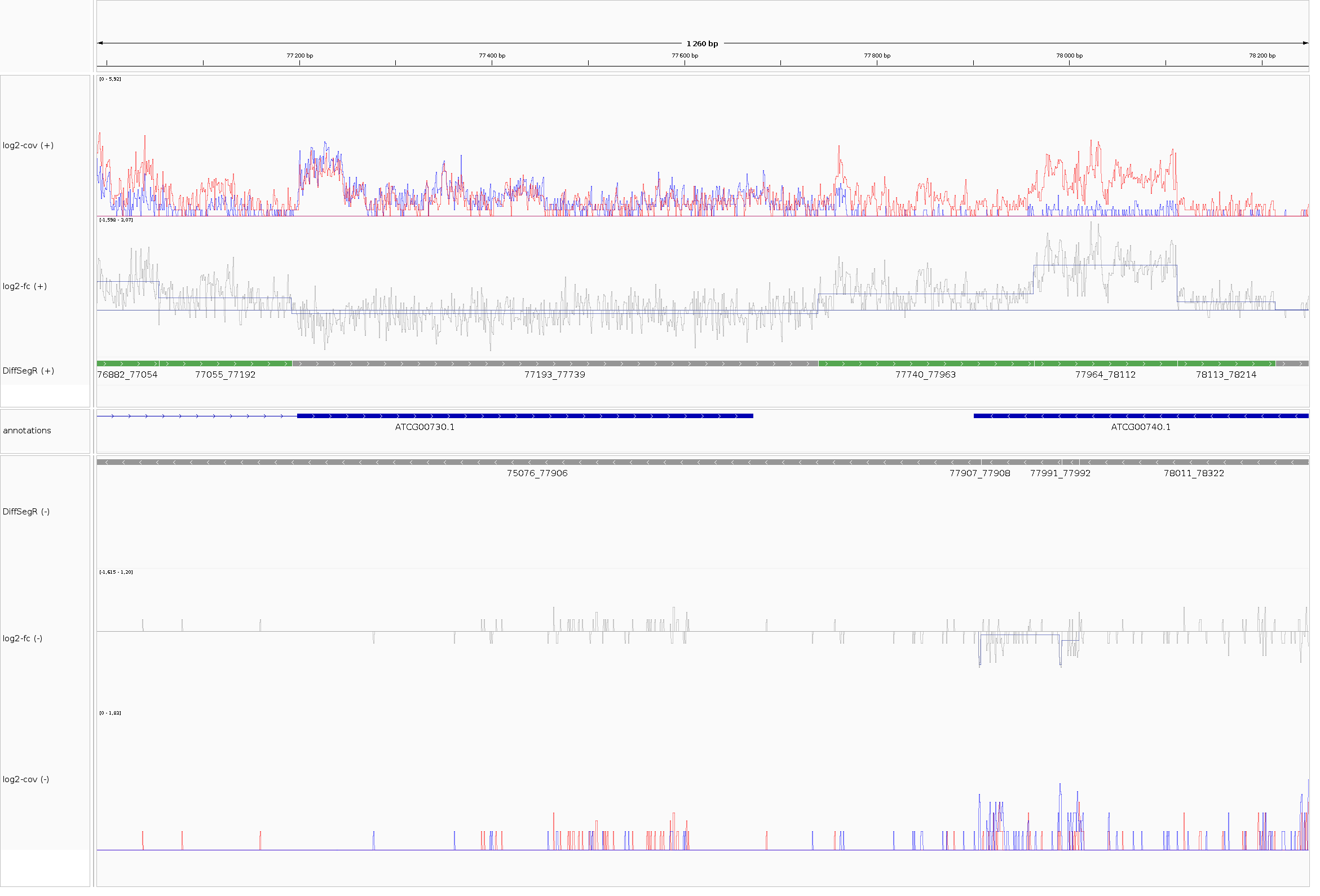
DiffSegR output between positions 76,990 to 78,248 on the chloroplast genome. The session is loaded in IGV 2.17.2 for Linux.
In collaboration projects, users will typically send the directory containing all tracks to collaborators. To load the session in IGV, the collaborator must update the paths for the genome and annotations in the XML file. This step may be necessary for each IGV session produced by a multi-loci analysis. To streamline this process, collaborators can modify all necessary paths directly from their R environment using the setPaths() function.
setPaths(
  directory = "collaborator_igv_session(s)_directory",
  genome    = "collaborator_genome_path",
  annotations = "collaborator_annotations_path"
)
References
Castandet B, Hotto AM, Fei Z, Stern DB. Strand-specific RNA sequencing uncovers chloroplast ribonuclease functions. FEBS Lett 587(18), 3096-101 (2013) doi:10.1016/j.febslet.2013.08.004.
Hotto AM, Castandet B, Gilet L, Higdon A, Condon C, Stern DB. Arabidopsis chloroplast mini-ribonuclease III participates in rRNA maturation and intron recycling. Plant Cell 27(3), 724-40 (2015) doi:10.1105/tpc.114.134452.
James T. Robinson, Helga Thorvaldsdóttir, Wendy Winckler, Mitchell Guttman, Eric S. Lander, Gad Getz, Jill P. Mesirov. Integrative Genomics Viewer. Nature Biotechnology 29, 24–26 (2011) doi:10.1038/nbt.1754.